

meta data for this page
Green Drive in Parallel drive

With the Green Drive Motor, you can drive two motors in parallel using only one encoder and one amplifier. All other systems require two drives, two controllers, and two encoders connected together.
The major issue with all parallel drive systems (e.g. gantries) is orthogonal alignment — the ability to keep the parallel axes square. In mechanical drive systems (screw-driven, rack-and-pinion, belt, and chain drive, to name a few), the main problem is binding of the system due to misalignment or stacked-up tolerances. In direct-drive systems, there is an additional issue: sine error, introduced by installation errors and by variances in the linear motors themselves.
The common way to overcome these issues is to drive and control each side of the parallel system separately and then synchronize them electronically. However, such a system costs more, since it requires twice the electronics (drivers and feedback, etc.) compared to a single-axis system. This tracking-control approach can also add synchronization and tracking errors, which adversely affect the performance of the system.
Sine Error
Sine error is the force difference produced by misalignment of a motor's coils or magnetic tracks.

In linear motors, current is applied to the coil to form an electromagnet. The coil then synchronizes itself to the magnetic field generated by the permanent magnets in the magnet track. Force is generated by the relative strength of these magnetic fields and by the angle of their intentional misalignment.
In a parallel drive system, when the magnetic fields of all the coils are perfectly aligned and the magnetic fields of all the magnet tracks are perfectly aligned, the two motors behave — in effect — as a single motor with no difference in force generation. However, any misalignment of the coils or the magnetic tracks makes the misalignment angle of the magnetic fields differ between the motors, producing different forces in each. This force difference can, in turn, cause binding in the system.
Sine error can be calculated with the following formula:

where Fdif is the force difference between the two coils, Fgen the force generated, Dfid the length of misalignment, and MPn-n the pole pitch (N-N). Most linear motors are designed with a north-to-north magnetic pitch in the range of 25 to 60 mm, in order to reduce IR losses and the electrical time constant.
For example, a misalignment of just 1 mm in a linear motor with a 30 mm N-N pitch causes a loss of about 21 percent of its power. On the other hand, the Linear Shaft Motor uses a much longer north-to-north magnetic pitch to reduce the effect of sine error caused by accidental misalignment. Therefore, the same 1 mm misalignment in a Linear Shaft Motor with a 90 mm N-N pitch results in only a 7 percent loss of power.
How to mount the motor to avoid sine error
The forcers and shafts in a parallel drive system must be physically coupled by a mechanism that allows the moving axis to realize one-degree-of-freedom movement.

Both forcers must be oriented in the same direction on their shafts. It is recommended that the end of the forcer carrying the serial number points toward the end of the shaft marked with yellow paint. If the orientation of the coils differs, the system may become totally inoperable or runaway, or it will cause significant loss of thrust. The standard for a parallel drive system is mirrored cable exit locations. See the drawing below.

How to find the orientation of the shaft without marking
Using a screwdriver, check the positioning of the first magnet inside the slider. The screwdriver will be attracted by the magnetic field of the magnets.
 | 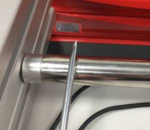 |
| Position when the magnets start. (close to the shaft end) Yellow point is on this side | Position when the magnets end. (away from the shaft end) |
Deviation in mounting the motors
To minimize loss of thrust due to sine error, it is recommended that the mounting position difference between the Linear Shaft Motors [Δx = Δx1 − Δx2] be less than the values shown in the table below.

| Model | Max Δx Δx = Δx1 − Δx2 [mm] | Minimal distance P [mm] |
| GD160 | 0.83 | 60 |
| GD250 | 1.25 | 90 |
| GD350 | 1.67 | 120 |